Beautiful Tips About How To Draw Pie Chart In Excel

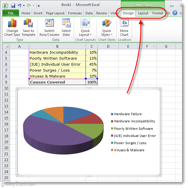
Excel 3-d Pie Charts - Microsoft 2016
/ExplodeChart-5bd8adfcc9e77c0051b50359.jpg)
How To Create Exploding Pie Charts In Excel

How To Make A Pie Chart In Excel
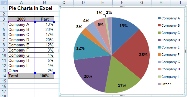
How To Create A Pie Chart In Excel (with Percentages) - Youtube
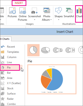
Add A Pie Chart
How To Create A Pie Chart In Excel And Google Sheets
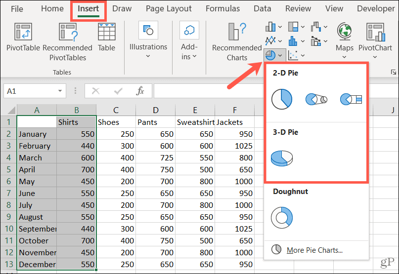
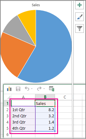
In the “insert” tab, from the “charts” section, select the “insert pie or doughnut chart” option (it’s.
How to draw pie chart in excel. Add data labels and data callouts to the pie chart. A list of options appears. In excel, click on the insert tab.
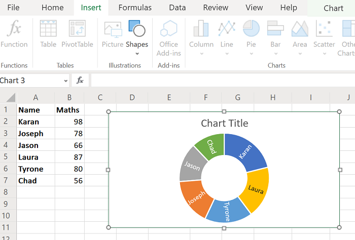
Now, from the insert tab >> you need to select insert pie or doughnut chart. How to create a pie chart in excel (with percentages) | simple pie chart in microsoft excel. Separate a few slices from the pie.
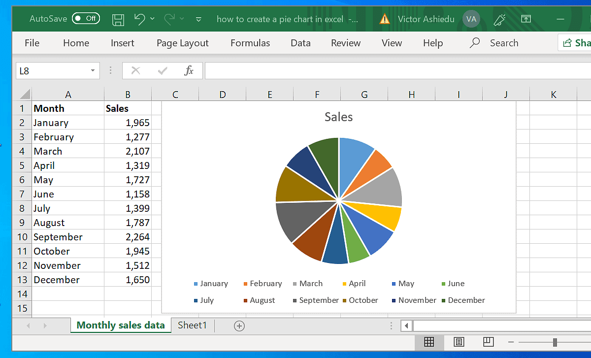
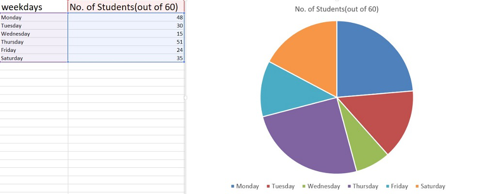
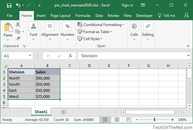
To create a pie chart, highlight the data in cells a3 to b6 and follow these directions: Download the sample spreadsheet used in this video from the following page: In the charts group, click insert pie or doughnut chart:
At the end, i also show you how. Pie chart is a circular statistical graphic which is divided into slices with numerical proportion it has been achieving great. Using a graph is a great way to present your data in an effective, visual way.
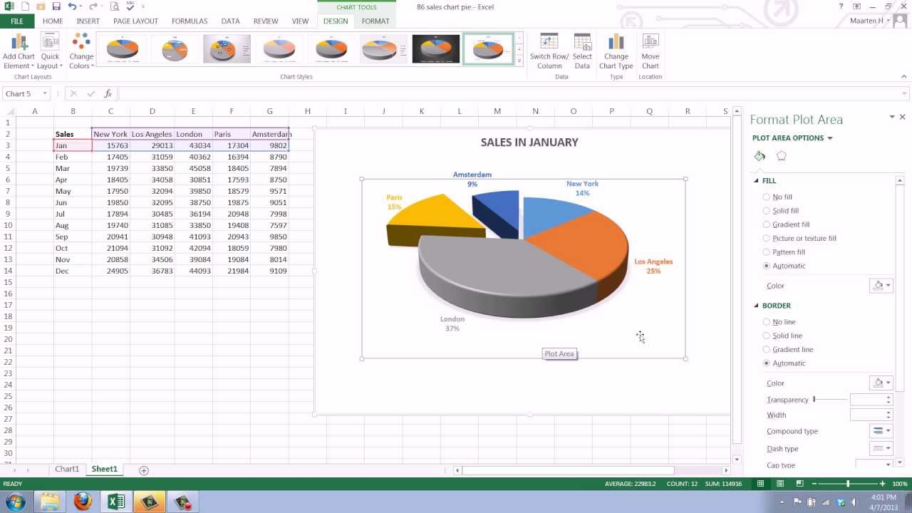
In the format data seriesdialog, click the drop down list besidesplit series byto selectpercentage value, and then set the value you want to display in the second pie, in this example, i will. How to create pie chart in microsoft excel. The steps to add percentages to the pie chart are:
Create a chart based on your first sheet. At this time, you will see the corresponding. Choose one of the graph and chart.
Follow the below steps to create a pie of pie chart: Excel 2010 how to create a pie chart. You can change the colour of each slice of your pie chart, and even move a slice the.
You can ctrl+click multiple graphics in the pane that appears on the right. From the dropdown menu that appears, select the bar of. Select insert pie chart to display the available.
On the drawing tools format tab, click the align button in the arrange group. To create a pie chart in excel 2016, add your data set to a worksheet and highlight it. Open your first excel worksheet, select the data you want to plot in the chart, go to the insert tab > charts group, and choose the chart.
If you forget which button is which, hover over each one, and excel will tell you which type of. From the insert tab, select the drop down arrow next to ‘insert pie or doughnut chart’. Click on the pie chart > click the ‘ + ’ icon > check/tick the “ data labels ” checkbox in the “ chart element ” box > select the “ data.

Create Outstanding Pie Charts In Excel | Pryor Learning
How To Make A Pie Chart In Excel Using Spreadsheet Data
How To Create A Pie Chart In Excel 2013 - Youtube
How To Make A Pie Chart In Microsoft Excel 2010 Or 2007
How To Create A Pie Chart In Excel 60 Seconds Or Less
How To Make A Pie Chart In Excel? - Geeksforgeeks
How To Create A Pie Chart In Excel | Smartsheet
Ms Excel 2016: How To Create A Pie Chart
Add A Pie Chart

Excel Pie Chart - Introduction To How Make A In Youtube

How To Make A Pie Chart In Excel
Creating Pie Of And Bar Charts - Microsoft Excel 2007